EPS: Eigenvalue Problem Solver

The Eigenvalue Problem Solver (EPS) is the main object provided by SLEPc. It is used to specify a linear eigenvalue problem, either in standard or generalized form, and provides uniform and efficient access to all of the linear eigensolvers included in the package. Conceptually, the level of abstraction occupied by EPS is similar to other solvers in PETSc such as KSP for solving linear systems of equations.

Eigenvalue Problems

In this section, we briefly present some basic concepts about eigenvalue problems as well as general techniques used to solve them. The description is not intended to be exhaustive. The objective is simply to define terms that will be referred to throughout the rest of the manual. Readers who are familiar with the terminology and the solution approach can skip this section. For a more comprehensive description, we refer the reader to monographs such as [Stewart, 2001], [Bai et al., 2000], [Saad, 1992] or [Parlett, 1980]. A historical perspective of the topic can be found in [Golub and van der Vorst, 2000]. See also the SLEPc technical reports.

In the standard formulation, the linear eigenvalue problem consists in the determination of \(\lambda\in\mathbb{C}\) for which the equation

(1)\[ Ax=\lambda x\]

has nontrivial solution, where \(A\in\mathbb{C}^{n\times n}\) and \(x\in\mathbb{C}^n\). The scalar \(\lambda\) and the vector \(x\) are called eigenvalue and (right) eigenvector, respectively. Note that they can be complex even when the matrix is real. If \(\lambda\) is an eigenvalue of \(A\) then \(\bar{\lambda}\) is an eigenvalue of its conjugate transpose, \(A^*\), or equivalently

(2)\[y^*\!A=\lambda\, y^*,\]

where \(y\) is called the left eigenvector.

In many applications, the problem is formulated as

(3)\[Ax=\lambda Bx,\]

where \(B\in\mathbb{C}^{n\times n}\), which is known as the generalized eigenvalue problem. Usually, this problem is solved by reformulating it in standard form, for example \(B^{-1}Ax=\lambda x\) if \(B\) is non-singular.

SLEPc focuses on the solution of problems in which the matrices are large and sparse. Hence, only methods that preserve sparsity are considered. These methods obtain the solution from the information generated by the application of the operator to various vectors (the operator is a simple function of matrices \(A\) and \(B\)), that is, matrices are only used in matrix-vector products. This not only maintains sparsity but allows the solution of problems in which matrices are not available explicitly.

In practical analyses, from the \(n\) possible solutions, typically only a few eigenpairs \((\lambda,x)\) are considered relevant, either in the extremities of the spectrum, in an interval, or in a region of the complex plane. Depending on the application, either eigenvalues or eigenvectors (or both) are required. In some cases, left eigenvectors are also of interest.

Projection Methods.

Most eigensolvers provided by SLEPc perform a Rayleigh-Ritz projection for extracting the spectral approximations, that is, they project the problem onto a low-dimensional subspace that is built appropriately. Suppose that an orthogonal basis of this subspace is given by \(V_j=[v_1,v_2,\ldots,v_j]\). If the solutions of the projected (reduced) problem \(B_js=\theta s\) (i.e., \(V_j^TAV_j=B_j\)) are assumed to be \((\theta_i,s_i)\), \(i=1,2,\ldots,j\), then the approximate eigenpairs \((\tilde{\lambda}_i,\tilde{x}_i)\) of the original problem (Ritz value and Ritz vector) are obtained as

(4)\[\begin{split}\begin{aligned} \tilde{\lambda}_i=\theta_i,\\ \end{aligned}\end{split}\]

(5)\[\begin{aligned} \tilde{x}_i=V_js_i. \end{aligned}\]

Starting from this general idea, eigensolvers differ from each other in which subspace is used, how it is built and other technicalities aimed at improving convergence, reducing storage requirements, etc.

The subspace

(6)\[\mathcal{K}_m(A,v)\equiv\mathrm{span}\left\{v,Av,A^2v,\ldots,A^{m-1}v\right\},\]

is called the \(m\)-th Krylov subspace corresponding to \(A\) and \(v\). Methods that use subspaces of this kind to carry out the projection are called Krylov methods. One example of such methods is the Arnoldi algorithm: starting with \(v_1\), \(\|v_1\|_2=1\), the Arnoldi basis generation process can be expressed by the recurrence

(7)\[v_{j+1}h_{j+1,j}=w_j=Av_j-\sum_{i=1}^jh_{i,j}v_i,\]

where \(h_{i,j}\) are the scalar coefficients obtained in the Gram-Schmidt orthogonalization of \(Av_j\) with respect to \(v_i\), \(i=1,2,\ldots,j\), and \(h_{j+1,j}=\|w_j\|_2\). Then, the columns of \(V_j\) span the Krylov subspace \(\mathcal{K}_j(A,v_1)\) and \(Ax=\lambda x\) is projected into \(H_js=\theta s\), where \(H_j\) is an upper Hessenberg matrix with elements \(h_{i,j}\), which are 0 for \(i\geq j+2\). The related Lanczos algorithms obtain a projected matrix that is tridiagonal.

A generalization to the above methods are the block Krylov strategies, in which the starting vector \(v_1\) is replaced by a full rank \(n\times p\) matrix \(V_1\), which allows for better convergence properties when there are multiple eigenvalues and can provide better data management on some computer architectures. Block tridiagonal and block Hessenberg matrices are then obtained as projections.

It is generally assumed (and observed) that the Lanczos and Arnoldi algorithms find solutions at the extremities of the spectrum. Their convergence pattern, however, is strongly related to the eigenvalue distribution. Slow convergence may be experienced in the presence of tightly clustered eigenvalues. The maximum allowable \(j\) may be reached without having achieved convergence for all desired solutions. Then, restarting is usually a useful technique and different strategies exist for that purpose. However, convergence can still be very slow and acceleration strategies must be applied. Usually, these techniques consist in computing eigenpairs of a transformed operator and then recovering the solution of the original problem. The aim of these transformations is twofold. On one hand, they make it possible to obtain eigenvalues other than those lying in the periphery of the spectrum. On the other hand, the separation of the eigenvalues of interest is improved in the transformed spectrum thus leading to faster convergence. The most commonly used spectral transformation is called shift-and-invert, which works with operator \((A-\sigma I)^{-1}\). It allows the computation of eigenvalues closest to \(\sigma\) with very good separation properties. When using this approach, a linear system of equations, \((A-\sigma I)y=x\), must be solved in each iteration of the eigenvalue process.

Preconditioned Eigensolvers

In many applications, Krylov eigensolvers perform very well because Krylov subspaces are optimal in a certain theoretical sense. However, these methods may not be appropriate in some situations such as the computation of interior eigenvalues. The spectral transformation mentioned above may not be a viable solution or it may be too costly. For these reasons, other types of eigensolvers such as Davidson and Jacobi-Davidson rely on a different way of expanding the subspace. Instead of satisfying the Krylov relation, these methods compute the new basis vector by the so-called correction equation. The resulting subspace may be richer in the direction of the desired eigenvectors. These solvers may be competitive especially for computing interior eigenvalues. From a practical point of view, the correction equation may be seen as a cheap replacement for the shift-and-invert system of equations, \((A-\sigma I)y=x\). By cheap we mean that it may be solved inaccurately without compromising robustness, via a preconditioned iterative linear solver. For this reason, these are known as preconditioned eigensolvers.

Related Problems

In many applications such as the analysis of damped vibrating systems the problem to be solved is a polynomial eigenvalue problem (PEP), or more generally a nonlinear eigenvalue problem (NEP). For these, the reader is referred to chapters PEP: Polynomial Eigenvalue Problems and NEP: Nonlinear Eigenvalue Problems. Another linear algebra problem that is very closely related to the eigenvalue problem is the singular value decomposition (SVD), see chapter SVD: Singular Value Decomposition.

Basic Usage

The EPS module in SLEPc is used in a similar way as PETSc modules such as KSP. All the information related to an eigenvalue problem is handled via a context variable. The usual object management functions are available (EPSCreate, EPSDestroy, EPSView, EPSSetFromOptions). In addition, the EPS object provides functions for setting several parameters such as the number of eigenvalues to compute, the dimension of the subspace, the portion of the spectrum of interest, the requested tolerance or the maximum number of iterations allowed.

The solution of the problem is obtained in several steps. First of all, the matrices associated with the eigenproblem are specified via EPSSetOperators and EPSSetProblemType is used to specify the type of problem. Then, a call to EPSSolve is done that invokes the subroutine for the selected eigensolver. EPSGetConverged can be used afterwards to determine how many of the requested eigenpairs have converged to working accuracy. EPSGetEigenpair is finally used to retrieve the eigenvalues and eigenvectors.

In order to illustrate the basic functionality of the EPS package, a simple example is shown in figure Example code for basic solution with EPS. The example code implements the solution of a simple standard eigenvalue problem. Code for setting up the matrix \(A\) is not shown and error-checking code is omitted.

Example code for basic solution with EPS

EPS         eps;       /*  eigensolver context  */
Mat         A;         /*  matrix of Ax=kx      */
Vec         xr, xi;    /*  eigenvector, x       */
PetscScalar kr, ki;    /*  eigenvalue, k        */
PetscInt    j, nconv;
PetscReal   error;

EPSCreate( PETSC_COMM_WORLD, &eps );
EPSSetOperators( eps, A, NULL );
EPSSetProblemType( eps, EPS_NHEP );
EPSSetFromOptions( eps );
EPSSolve( eps );
EPSGetConverged( eps, &nconv );
for (j=0; j<nconv; j++) {
  EPSGetEigenpair( eps, j, &kr, &ki, xr, xi );
  EPSComputeError( eps, j, EPS_ERROR_RELATIVE, &error );
}
EPSDestroy( &eps );

All the operations of the program are done over a single EPS object. This solver context is created in line 8 of Example code for basic solution with EPS with the command EPSCreate

EPSCreate(MPI_Comm comm,EPS *eps);

Here comm is the MPI communicator, and eps is the newly formed solver context. The communicator indicates which processes are involved in the EPS object. Most of the EPS operations are collective, meaning that all the processes collaborate to perform the operation in parallel.

Before actually solving an eigenvalue problem with EPS, the user must specify the matrices associated with the problem, as in line 9 of Example code for basic solution with EPS, with the following routine EPSSetOperators

EPSSetOperators(EPS eps,Mat A,Mat B);

The example specifies a standard eigenproblem. In the case of a generalized problem, it would be necessary also to provide matrix \(B\) as the third argument to the call. The matrices specified in this call can be in any PETSc format. In particular, EPS allows the user to solve matrix-free problems by specifying matrices created via MatCreateShell. A more detailed discussion of this issue is given in section Supported Matrix Types.

After setting the problem matrices, the problem type is set with EPSSetProblemType. This is not strictly necessary since if this step is skipped then the problem type is assumed to be non-symmetric. More details are given in section Defining the Problem. At this point, the value of the different options could optionally be set by means of a function call such as EPSSetTolerances (explained later in this chapter). After this, a call to EPSSetFromOptions should be made as in line 11 of Example code for basic solution with EPS, EPSSetFromOptions

EPSSetFromOptions(EPS eps);

The effect of this call is that options specified at runtime in the command line are passed to the EPS object appropriately. In this way, the user can easily experiment with different combinations of options without having to recompile. All the available options as well as the associated function calls are described later in this chapter.

Line 12 launches the solution algorithm, simply with the command EPSSolve

EPSSolve(EPS eps);

The subroutine that is actually invoked depends on which solver has been selected by the user.

After the call to EPSSolve has finished, all the data associated with the solution of the eigenproblem are kept internally. This information can be retrieved with different function calls, as in lines 13 to 17 of Example code for basic solution with EPS. This part is described in detail in section Retrieving the Solution.

Once the EPS context is no longer needed, it should be destroyed with the command EPSDestroy

EPSDestroy(EPS *eps);

The above procedure is sufficient for general use of the EPS package. As in the case of the KSP solver, the user can optionally explicitly call EPSSetUp

EPSSetUp(EPS eps);

before calling EPSSolve to perform any setup required for the eigensolver.

Internally, the EPS object works with an ST object (spectral transformation, described in chapter ST: Spectral Transformation. To allow application programmers to set any of the spectral transformation options directly within the code, the following routine is provided to extract the ST context, EPSGetST

EPSGetST(EPS eps,ST *st);

With the command EPSView

EPSView(EPS eps,PetscViewer viewer);

it is possible to examine the actual values of the different settings of the EPS object, including also those related to the associated ST object. This is useful for making sure that the solver is using the settings that the user wants.

Defining the Problem

SLEPc is able to cope with different kinds of problems. Currently supported problem types are listed in table Problem types considered in EPS.. An eigenproblem is generalized (\(Ax=\lambda Bx\)) if the user has specified two matrices (see EPSSetOperators above), otherwise it is standard (\(Ax=\lambda x\)). A standard eigenproblem is Hermitian if matrix \(A\) is Hermitian (i.e., \(A=A^*\)) or, equivalently in the case of real matrices, if matrix \(A\) is symmetric (i.e., \(A=A^T\)). A generalized eigenproblem is Hermitian if matrix \(A\) is Hermitian (symmetric) and \(B\) is Hermitian (symmetric) and positive (semi-)definite. If \(B\) is not positive (semi-)definite then the problem cannot be considered Hermitian but symmetry can still be exploited to some extent in some solvers (problem type EPS_GHIEP). A special case of generalized non-Hermitian problem is when \(A\) is non-Hermitian but \(B\) is Hermitian and positive (semi-)definite, see section Preserving the Symmetry in Generalized Eigenproblems and Purification of Eigenvectors for discussion. The last entries in table Problem types considered in EPS., separated by a line, correspond to structured eigenvalue problems, which are discussed in section Structured Eigenvalue Problems.

Problem types considered in EPS.

Problem Type	EPSProblemType	Command line key
Hermitian	EPS_HEP	-eps_hermitian
Non-Hermitian	EPS_NHEP	-eps_non_hermitian
Generalized Hermitian	EPS_GHEP	-eps_gen_hermitian
Generalized Hermitian indefinite	EPS_GHIEP	-eps_gen_indefinite
Generalized Non-Hermitian	EPS_GNHEP	-eps_gen_non_hermitian
GNHEP with positive (semi-)definite \(B\)	EPS_PGNHEP	-eps_pos_gen_non_hermitian
Bethe-Salpeter	EPS_BSE	-eps_bse
Hamiltonian	EPS_HAMILT	-eps_hamiltonian

The problem type can be specified at run time with the corresponding command line key or, more usually, within the program with the function EPSSetProblemType

EPSSetProblemType(EPS eps,EPSProblemType type);

By default, SLEPc assumes that the problem is non-Hermitian. Some eigensolvers are able to exploit symmetry, that is, they compute a solution for Hermitian problems with less storage and/or computational cost than other methods that ignore this property. Also, symmetric solvers may be more accurate. On the other hand, some eigensolvers in SLEPc only have a symmetric version and will abort if the problem is non-Hermitian. In the case of generalized eigenproblems some considerations apply regarding symmetry, especially in the case of singular \(B\). This topic is covered in section Preserving the Symmetry in Generalized Eigenproblems and Purification of Eigenvectors. Similarly, if your eigenproblem has a particular algebraic structure listed in table Problem types considered in EPS., solving it with a structured eigensolver as discussed in section Structured Eigenvalue Problems will result in more accuracy and better efficiency. For all these reasons, the user is strongly recommended to always specify the problem type in the source code.

The characteristics of the problem can be determined with the functions EPSIsGeneralized EPSIsHermitian EPSIsPositive EPSIsStructured

EPSIsGeneralized(EPS eps,PetscBool *gen);
EPSIsHermitian(EPS eps,PetscBool *her);
EPSIsPositive(EPS eps,PetscBool *pos);
EPSIsStructured(EPS eps,PetscBool *stru);

The user can specify how many eigenvalues (and eigenvectors) to compute. The default is to compute only one. The function EPSSetDimensions

EPSSetDimensions(EPS eps,PetscInt nev,PetscInt ncv,PetscInt mpd);

allows the specification of the number of eigenvalues to compute, nev. The next argument can be set to prescribe the number of column vectors to be used by the solution algorithm, ncv, that is, the largest dimension of the working subspace. The last argument has to do with a more advanced usage, as explained in section Computing a Large Portion of the Spectrum. These parameters can also be set at run time with the options -eps_nev, -eps_ncv and -eps_mpd. For example, the command line

$ ./program -eps_nev 10 -eps_ncv 24

requests 10 eigenvalues and instructs to use 24 column vectors. Note that ncv must be at least equal to nev, although in general it is recommended (depending on the method) to work with a larger subspace, for instance \(\mathtt{ncv}\geq2\cdot\mathtt{nev}\) or even more. The case that the user requests a relatively large number of eigenpairs is discussed in section Computing a Large Portion of the Spectrum.

Instead of specifying the number of wanted eigenvalues nev, it is also possible to specify a threshold with EPSSetThreshold

EPSSetThreshold(EPS eps,PetscReal thres,PetscBool rel);

This usage is discussed in section Using a threshold to specify wanted singular values for the case of SVD. For details about the differences in case of EPS, we refer to the manual page of EPSSetThreshold.

Eigenvalues of Interest

For the selection of the portion of the spectrum of interest, there are several alternatives. In real symmetric problems, one may want to compute the largest or smallest eigenvalues in magnitude, or the leftmost or rightmost ones, or even all eigenvalues in a given interval. In other problems, in which the eigenvalues can be complex, then one can select eigenvalues depending on the magnitude, or the real part or even the imaginary part. Sometimes the eigenvalues of interest are those closest to a given target value, \(\tau\), measuring the distance either in the ordinary way or along the real (or imaginary) axis. In some other cases, wanted eigenvalues must be found in a given region of the complex plane. Table Available possibilities for selection of the eigenvalues of interest. summarizes all the possibilities available for the function EPSSetWhichEigenpairs

EPSSetWhichEigenpairs(EPS eps,EPSWhich which);

which can also be specified at the command line. This criterion is used both for configuring how the eigensolver seeks eigenvalues (note that not all these possibilities are available for all the solvers) and also for sorting the computed values. The default is to compute the largest magnitude eigenvalues, except for those solvers in which this option is not available. There is another exception related to the use of some spectral transformations, see chapter ST: Spectral Transformation.

For the sorting criteria relative to a target value, the following function must be called in order to specify such value \(\tau\): EPSSetTarget

EPSSetTarget(EPS eps,PetscScalar target);

or, alternatively, with the command-line key -eps_target. Note that, since the target is defined as a PetscScalar, complex values of \(\tau\) are allowed only in the case of complex scalar builds of the SLEPc library.

The use of a target value makes sense if the eigenvalues of interest are located in the interior of the spectrum. Since these eigenvalues are usually more difficult to compute, the eigensolver by itself may not be able to obtain them, and additional tools are normally required. There are two possibilities for this:

• To use harmonic extraction (see section Computing Interior Eigenvalues with Harmonic Extraction), a variant of some solvers that allows a better approximation of interior eigenvalues without changing the way the subspace is built.

• To use a spectral transformation such as shift-and-invert (see chapter ST: Spectral Transformation), where the subspace is built from a transformed problem (usually much more costly).

The special case of computing all eigenvalues in an interval is discussed in the next chapter (sections Polynomial Filtering and Spectrum Slicing), since it is related also to spectral transformations. In this case, instead of a target value the user has to specify the computational interval with EPSSetInterval

EPSSetInterval(EPS eps,PetscScalar a,PetscScalar b);

which is equivalent to -eps_interval a,b.

Available possibilities for selection of the eigenvalues of interest.

EPSWhich	Command line key	Sorting criterion
EPS_LARGEST_MAGNITUDE	-eps_largest_magnitude	Largest \(|\lambda|\)
EPS_SMALLEST_MAGNITUDE	-eps_smallest_magnitude	Smallest \(|\lambda|\)
EPS_LARGEST_REAL	-eps_largest_real	Largest \(\mathrm{Re}(\lambda)\)
EPS_SMALLEST_REAL	-eps_smallest_real	Smallest \(\mathrm{Re}(\lambda)\)
EPS_LARGEST_IMAGINARY	-eps_largest_imaginary	Largest \(\mathrm{Im}(\lambda)\)[1]
EPS_SMALLEST_IMAGINARY	-eps_smallest_imaginary	Smallest \(\mathrm{Im}(\lambda)\)[1]
EPS_TARGET_MAGNITUDE	-eps_target_magnitude	Smallest \(|\lambda-\tau|\)
EPS_TARGET_REAL	-eps_target_real	Smallest \(|\mathrm{Re}(\lambda-\tau)|\)
EPS_TARGET_IMAGINARY	-eps_target_imaginary	Smallest \(|\mathrm{Im}(\lambda-\tau)|\)
EPS_ALL	-eps_all	All \(\lambda\in[a,b]\) or \(\lambda\in\Omega\)
EPS_WHICH_USER		user-defined

There is also support for specifying a region of the complex plane so that the eigensolver finds eigenvalues within that region only. This possibility is described in section Specifying a Region for Filtering. If all eigenvalues inside the region are required, then a contour-integral method must be used, as described in Maeda et al. [2016].

Finally, we mention the possibility of defining an arbitrary sorting criterion by means of EPS_WHICH_USER in combination with EPSSetEigenvalueComparison.

The selection criteria discussed above are based solely on the eigenvalue. In some special situations, it is necessary to establish a user-defined criterion that also makes use of the eigenvector when deciding which are the most wanted eigenpairs. For these cases, use EPSSetArbitrarySelection.

Left Eigenvectors.

In addition to right eigenvectors, some solvers are able to compute also left eigenvectors, as defined in equation (2). The algorithmic variants that compute both left and right eigenvectors are usually called two-sided. By default, SLEPc computes right eigenvectors only. To compute also left eigenvectors, the user should set a flag by calling the following function before EPSSolve. EPSSetTwoSided

EPSSetTwoSided(EPS eps,PetscBool twosided);

Note that in some problems such as Hermitian or generalized Hermitian, the left eigenvector can be obtained trivially from the right eigenvector. In other cases such as non-Hermitian problems (either standard or generalized), the user must set the two-sided flag before the solver starts to compute, and this is restricted to just a few solvers, see table Supported problem types for all eigensolvers available in SLEPc..

Selecting the Eigensolver

The available methods for solving the eigenvalue problems are the following:

• Basic methods (not recommended except for simple problems):

  • Power Iteration with deflation. When combined with shift-and-invert (see chapter ST: Spectral Transformation), it is equivalent to the inverse iteration. Also, this solver embeds the Rayleigh Quotient iteration (RQI) by allowing variable shifts. Additionally, it provides the nonlinear inverse iteration method for the case that the problem matrix is a nonlinear operator (for this advanced usage, see EPSPowerSetNonlinear).

  • Subspace Iteration with Rayleigh-Ritz projection and locking.

  • Arnoldi method with explicit restart and deflation.

  • Lanczos with explicit restart, deflation, and different reorthogonalization strategies.

• Krylov-Schur, a variation of Arnoldi with a very effective restarting technique. In the case of symmetric problems, this is equivalent to the thick-restart Lanczos method.

• Generalized Davidson, a simple iteration based on subspace expansion with the preconditioned residual.

• Jacobi-Davidson, a preconditioned eigensolver with an effective correction equation.

• RQCG, a basic conjugate gradient iteration for the minimization of the Rayleigh quotient.

• LOBPCG, the locally-optimal block preconditioned conjugate gradient.

• CISS, a contour-integral solver that allows computing all eigenvalues in a given region.

• Lyapunov inverse iteration, to compute rightmost eigenvalues.

Eigenvalue solvers available in the EPS module.

Method	EPSType	Options Database Name	Default
Power / Inverse / RQI	EPSPOWER	power
Subspace Iteration	EPSSUBSPACE	subspace
Arnoldi	EPSARNOLDI	arnoldi
Lanczos	EPSLANCZOS	lanczos
Krylov-Schur	EPSKRYLOVSCHUR	krylovschur	\(\star\)
Generalized Davidson	EPSGD	gd
Jacobi-Davidson	EPSJD	jd
Rayleigh quotient CG	EPSRQCG	rqcg
LOBPCG	EPSLOBPCG	lobpcg
Contour integral SS	EPSCISS	ciss
Lyapunov Inverse Iteration	EPSLYAPII	lyapii
LAPACK solver	EPSLAPACK	lapack
Wrapper to ARPACK	EPSARPACK	arpack
Wrapper to PRIMME	EPSPRIMME	primme
Wrapper to EVSL	EPSEVSL	evsl
Wrapper to BLOPEX	EPSBLOPEX	blopex
Wrapper to ScaLAPACK	EPSSCALAPACK	scalapack
Wrapper to ELPA	EPSELPA	elpa
Wrapper to ELEMENTAL	EPSELEMENTAL	elemental
Wrapper to CHASE	EPSCHASE	chase
Wrapper to FEAST	EPSFEAST	feast

The default solver is Krylov-Schur. A detailed description of the implemented algorithms is provided in the SLEPc Technical Reports. In addition to these methods, SLEPc also provides wrappers to external packages such as ARPACK, or PRIMME. A complete list of these interfaces can be found in section Wrappers to External Libraries. Note that some of these packages (LAPACK, ScaLAPACK, ELPA, ELEMENTAL) perform dense computations and hence return the full eigendecomposition (furthermore, take into account that LAPACK is a sequential library so the corresponding solver should be used only for debugging purposes with small problem sizes).

The solution method can be specified procedurally or via the command line. The application programmer can set it by means of the command EPSSetType

EPSSetType(EPS eps,EPSType method);

while the user writes the options database command -eps_type followed by the name of the method (see table Eigenvalue solvers available in the EPS module.).

Not all the methods can be used for all problem types. Table Supported problem types for all eigensolvers available in SLEPc. summarizes the scope of each eigensolver by listing which portion of the spectrum can be selected (as defined in table Available possibilities for selection of the eigenvalues of interest.) and which problem types are supported (as defined in table Problem types considered in EPS.). Note that the structured problem types are not considered here, see section Structured Eigenvalue Problems. The table also indicates whether the solvers are available or not in the complex version of SLEPc, and if they have a two-sided variant.

Supported problem types for all eigensolvers available in SLEPc.

Method	Portion of spectrum	Problem type	Real/complex	Two-sided
power	Largest \(|\lambda|\)	any	both	yes
subspace	Largest \(|\lambda|\)	any	both
arnoldi	any	any	both
lanczos	any	EPS_HEP, EPS_GHEP	both
krylovschur	any	any	both	yes
gd	any	any	both
jd	any	any	both
rqcg	Smallest \(\mathrm{Re}(\lambda)\)	EPS_HEP, EPS_GHEP	both
lobpcg	Smallest \(\mathrm{Re}(\lambda)\)	EPS_HEP, EPS_GHEP	both
ciss	All \(\lambda\) in region	any	both
lyapii	Largest \(\mathrm{Re}(\lambda)\)	any	both
lapack	any	any	both	yes
arpack	any	any	both
primme	Largest and smallest \(\mathrm{Re}(\lambda)\)	EPS_HEP, EPS_GHEP	both
evsl	All \(\lambda\) in interval	EPS_HEP	real
blopex	Smallest \(\mathrm{Re}(\lambda)\)	EPS_HEP, EPS_GHEP	both
scalapack	All \(\lambda\)	EPS_HEP, EPS_GHEP	both
elpa	All \(\lambda\)	EPS_HEP, EPS_GHEP	both
elemental	All \(\lambda\)	EPS_HEP, EPS_GHEP	both
chase	Smallest \(\mathrm{Re}(\lambda)\)	EPS_HEP	both
feast	All \(\mathrm{Re}(\lambda)\) in an interval	any	both

Retrieving the Solution

Once the call to EPSSolve is complete, all the data associated with the solution of the eigenproblem are kept internally in the EPS object. This information can be obtained by the calling program by means of a set of functions described in this section.

As explained below, the number of computed solutions depends on the convergence and, therefore, it may be different from the number of solutions requested by the user. So the first task is to find out how many solutions are available, with EPSGetConverged

EPSGetConverged(EPS eps,PetscInt *nconv);

Usually, the number of converged solutions, nconv, will be equal to nev, but in general it can be a number ranging from 0 to ncv (here, nev and ncv are the arguments of function EPSSetDimensions).

The Computed Solution

The user may be interested in the eigenvalues, or the eigenvectors, or both. The function EPSGetEigenpair

EPSGetEigenpair(EPS eps,PetscInt j,PetscScalar *kr,PetscScalar *ki, Vec xr,Vec xi);

returns the \(j\)-th computed eigenvalue/eigenvector pair. Typically, this function is called inside a loop for each value of j from 0 to nconv–1. Note that eigenvalues are ordered according to the same criterion specified with function EPSSetWhichEigenpairs for selecting the portion of the spectrum of interest. The meaning of the last 4 arguments depends on whether SLEPc has been compiled for real or complex scalars, as detailed below. The eigenvectors are normalized so that they have a unit 2-norm, except for problem type EPS_GHEP in which case returned eigenvectors have a unit \(B\)-norm.

In case they are available, the left eigenvectors can be extracted with EPSGetLeftEigenvector

EPSGetLeftEigenvector(EPS eps,PetscInt j,Vec yr,Vec yi);

Real SLEPc

In this case, all Mat and Vec objects are real. The computed approximate solution returned by the function EPSGetEigenpair is stored in the following way: kr and ki contain the real and imaginary parts of the eigenvalue, respectively, and xr and xi contain the associated eigenvector. Two cases can be distinguished:

• When ki is zero, it means that the \(j\)-th eigenvalue is a real number. In this case, kr is the eigenvalue and xr is the corresponding eigenvector. The vector xi is set to all zeros.

• If ki is different from zero, then the \(j\)-th eigenvalue is a complex number and, therefore, it is part of a complex conjugate pair. Thus, the \(j\)-th eigenvalue is kr\(+\,i\cdot\)ki. With respect to the eigenvector, xr stores the real part of the eigenvector and xi the imaginary part, that is, the \(j\)-th eigenvector is xr\(+\,i\cdot\)xi. The \((j+1)\)-th eigenvalue (and eigenvector) will be the corresponding complex conjugate and will be returned when function EPSGetEigenpair is invoked with index j+1. Note that the sign of the imaginary part is returned correctly in all cases (users need not change signs).

Complex SLEPc

In this case, all Mat and Vec objects are complex. The computed solution returned by function EPSGetEigenpair is the following: kr contains the (complex) eigenvalue and xr contains the corresponding (complex) eigenvector. In this case, ki and xi are not used (set to all zeros).

Reliability of the Computed Solution

In this subsection, we discuss how a-posteriori error bounds can be obtained in order to assess the accuracy of the computed solutions. These bounds are based on the so-called residual vector, defined as

(8)\[r=A\tilde{x}-\tilde{\lambda}\tilde{x},\]

or \(r=A\tilde{x}-\tilde{\lambda}B\tilde{x}\) in the case of a generalized problem, where \(\tilde{\lambda}\) and \(\tilde{x}\) represent any of the nconv computed eigenpairs delivered by EPSGetEigenpair (note that this function returns a normalized \(\tilde{x}\)).

In the case of Hermitian problems, it is possible to demonstrate the following property (see for example [Saad, 1992, ch. 3]):

(9)\[|\lambda-\tilde{\lambda}|\leq \|r\|_2,\]

where \(\lambda\) is an exact eigenvalue. Therefore, the 2-norm of the residual vector can be used as a bound for the absolute error in the eigenvalue.

In the case of non-Hermitian problems, the situation is worse because no simple relation such as equation (9) is available. This means that in this case the residual norms may still give an indication of the actual error but the user should be aware that they may sometimes be completely wrong, especially in the case of highly non-normal matrices. A better bound would involve also the residual norm of the left eigenvector.

With respect to eigenvectors, we have a similar scenario in the sense that bounds for the error may be established in the Hermitian case only, for example the following one:

(10)\[\sin \theta(x,\tilde{x})\leq \frac{\|r\|_2}{\delta},\]

where \(\theta(x,\tilde{x})\) is the angle between the computed and exact eigenvectors, and \(\delta\) is the distance from \(\tilde{\lambda}\) to the rest of the spectrum. This bound is not provided by SLEPc because \(\delta\) is not available. The above expression is given here simply to warn the user about the fact that accuracy of eigenvectors may be deficient in the case of clustered eigenvalues.

In the case of non-Hermitian problems, SLEPc provides the alternative of retrieving an orthonormal basis of an invariant subspace instead of getting individual eigenvectors. This is done with function EPSGetInvariantSubspace

EPSGetInvariantSubspace(EPS eps,Vec v[]);

This is sufficient in some applications and is safer from the numerical point of view.

Computation of Bounds

It is sometimes useful to compute error bounds based on the norm of the residual \(r_j\), to assess the accuracy of the computed solution. The bound can be made in absolute terms, as in equation (9), or alternatively the error can be expressed relative to the eigenvalue or to the matrix norms. For this, the following function can be used: EPSComputeError

EPSComputeError(EPS eps,PetscInt j,EPSErrorType type,PetscReal *error);

The types of errors that can be computed are summarized in table Available expressions for computing error bounds.. The way in which the error is computed is unrelated to the error estimation used internally in the solver for convergence checking, as described below. Also note that in the case of two-sided eigensolvers, the error bounds are based on \(\max\{\|\ell_j\|,\|r_j\|\}\), where the left residual \(\ell_j\) is defined as \(\ell_j=A^*\tilde{y}-\bar{\tilde\lambda}\tilde{y}\).

Available expressions for computing error bounds.

Error type	EPSErrorType	Command line key	Error bound
Absolute error	EPS_ERROR_ABSOLUTE	-eps_error_absolute	\(|r|\)
Relative error	EPS_ERROR_RELATIVE	-eps_error_relative	\(|r|/|\lambda|\)
Backward error	EPS_ERROR_BACKWARD	-eps_error_backward	\(|r|/(|A|+|\lambda||B|)\)

Controlling and Monitoring Convergence

All the eigensolvers provided by SLEPc are iterative in nature, meaning that the solutions are (usually) improved at each iteration until they are sufficiently accurate, that is, until convergence is achieved. The number of iterations required by the process can be obtained with the function EPSGetIterationNumber

EPSGetIterationNumber(EPS eps,PetscInt *its);

which returns in argument its either the iteration number at which convergence was successfully reached, or the iteration at which a problem was detected.

The user specifies when a solution should be considered sufficiently accurate by means of a tolerance. An approximate eigenvalue is considered to be converged if the error estimate associated with it is below the specified tolerance. The default value of the tolerance is \(10^{-8}\) and can be changed at run time with -eps_tol <tol> or inside the program with the function EPSSetTolerances

EPSSetTolerances(EPS eps,PetscReal tol,PetscInt max_it);

The third parameter of this function allows the programmer to modify the maximum number of iterations allowed to the solution algorithm, which can also be set via -eps_max_it <its>.

Convergence Check

The error estimates used for the convergence test are based on the residual norm, as discussed in section Reliability of the Computed Solution. Most eigensolvers explicitly compute the residual of the relevant eigenpairs during the iteration, but Krylov solvers use a cheap formula instead, allowing to track many eigenpairs simultaneously. When using a spectral transformation, this formula may give too optimistic bounds (corresponding to the residual of the transformed problem, not the original problem). In such cases, the users can force the computation of the residual with EPSSetTrueResidual

EPSSetTrueResidual(EPS eps,PetscBool trueres);

or with -eps_true_residual.

Available possibilities for the convergence criterion.

Convergence criterion	EPSConv	Command line key	Error bound
Absolute	EPS_CONV_ABS	-eps_conv_abs	\(|r|\)
Relative to eigenvalue	EPS_CONV_REL	-eps_conv_rel	\(|r|/|\lambda|\)
Relative to matrix norms	EPS_CONV_NORM	-eps_conv_norm	\(|r|/(|A|+|\lambda||B|)\)
User-defined	EPS_CONV_USER	-eps_conv_user	user function

From the residual norm, the error bound can be computed in different ways, see table Available possibilities for the convergence criterion.. This can be set via the corresponding command-line switch or with EPSSetConvergenceTest

EPSSetConvergenceTest(EPS eps,EPSConv conv);

The default is to use the criterion relative to the eigenvalue (note: for computing eigenvalues close to the origin this criterion will likely give very poor accuracy, so the user is advised to use EPS_CONV_ABS in that case). Finally, a custom convergence criterion may be established by specifying a user function (EPSSetConvergenceTestFunction).

Error estimates used internally by eigensolvers for checking convergence may be different from the error bounds provided by EPSComputeError. At the end of the solution process, error estimates are available via EPSGetErrorEstimate

EPSGetErrorEstimate(EPS eps,PetscInt j,PetscReal *errest);

By default, the eigensolver will stop iterating when the current number of eigenpairs satisfying the convergence test is equal to (or greater than) the number of requested eigenpairs (or if the maximum number of iterations has been reached). However, it is also possible to provide a user-defined stopping test that may decide to quit earlier, see EPSSetStoppingTest.

Monitors

Error estimates can be displayed during execution of the solution algorithm, as a way of monitoring convergence. There are several such monitors available. The user can activate them via the options database (see examples below), or within the code with EPSMonitorSet. By default, the solvers run silently without displaying information about the iteration. Also, application programmers can provide their own routines to perform the monitoring by using the function EPSMonitorSet.

The most basic monitor prints one approximate eigenvalue together with its associated error estimate in each iteration. The shown eigenvalue is the first unconverged one.

$ ./ex9 -eps_nev 1 -eps_tol 1e-6 -eps_monitor

     1 EPS nconv=0 first unconverged value (error) -0.0695109+2.10989i (2.38956768e-01)
     2 EPS nconv=0 first unconverged value (error) -0.0231046+2.14902i (1.09212525e-01)
     3 EPS nconv=0 first unconverged value (error) -0.000633399+2.14178i (2.67086904e-02)
     4 EPS nconv=0 first unconverged value (error) 9.89074e-05+2.13924i (6.62097793e-03)
     5 EPS nconv=0 first unconverged value (error) -0.000149404+2.13976i (1.53444214e-02)
     6 EPS nconv=0 first unconverged value (error) 0.000183676+2.13939i (2.85521004e-03)
     7 EPS nconv=0 first unconverged value (error) 0.000192479+2.13938i (9.97563492e-04)
     8 EPS nconv=0 first unconverged value (error) 0.000192534+2.13938i (1.77259863e-04)
     9 EPS nconv=0 first unconverged value (error) 0.000192557+2.13938i (2.82539990e-05)
    10 EPS nconv=0 first unconverged value (error) 0.000192559+2.13938i (2.51440008e-06)
    11 EPS nconv=2 first unconverged value (error) -0.671923+2.52712i (8.92724972e-05)

Graphical monitoring (in an X display) is also available with -eps_monitor draw::draw_lg. Figure Monitor shows the result of the following sample command line:

$ ./ex9 -n 200 -eps_nev 12 -eps_tol 1e-12 -eps_monitor draw::draw_lg -draw_pause .2

Again, only the error estimate of one eigenvalue is drawn. The spikes in the last part of the plot indicate convergence of one eigenvalue and switching to the next.

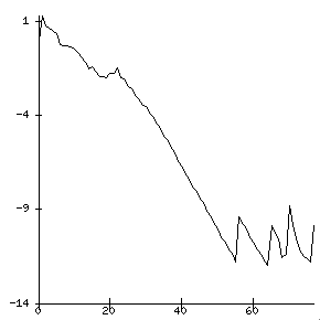
Default convergence monitor.

The two previously mentioned monitors have an alternative version (*_all) that processes all eigenvalues instead of just the first one. Figure Monitor-all corresponds to the same example but with -eps_monitor_all draw::draw_lg. Note that these variants have a side effect: they force the computation of all error estimates even if the method would not normally do so.

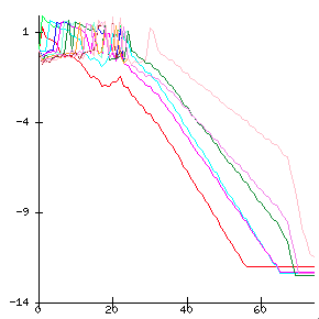
Simultaneous convergence monitor for all eigenvalues.

A less verbose monitor is -eps_monitor_conv, which simply displays the iteration number at which convergence takes place. Note that several monitors can be used at the same time.

$ ./ex9 -n 200 -eps_nev 8 -eps_tol 1e-12 -eps_monitor_conv

    79 EPS converged value (error) #0 4.64001e-06+2.13951i (8.26091148e-13)
    79 EPS converged value (error) #1 4.64001e-06-2.13951i (8.26091148e-13)
    93 EPS converged value (error) #2 -0.674926+2.52867i (6.85260521e-13)
    93 EPS converged value (error) #3 -0.674926-2.52867i (6.85260521e-13)
    94 EPS converged value (error) #4 -1.79963+3.03259i (5.48825386e-13)
    94 EPS converged value (error) #5 -1.79963-3.03259i (5.48825386e-13)
    98 EPS converged value (error) #6 -3.37383+3.55626i (2.74909207e-13)
    98 EPS converged value (error) #7 -3.37383-3.55626i (2.74909207e-13)

Viewing the Solution

The computed solution (eigenvalues and eigenvectors) can be viewed in different ways, exploiting the flexibility of PetscViewers. The API functions for this are EPSValuesView and EPSVectorsView. We next illustrate their usage via the command line.

The command-line option -eps_view_values shows the computed eigenvalues on the standard output at the end of EPSSolve. It admits an argument to specify PetscViewer options, for instance the following will create a Matlab command file myeigenvalues.m to load the eigenvalues in Matlab:

$ ./ex1 -n 120 -eps_nev 8 -eps_view_values :myeigenvalues.m:ascii_matlab

Lambda_EPS_0xb430f0_0 = [
3.9993259306070224e+00
3.9973041767976509e+00
3.9939361013742269e+00
3.9892239746533216e+00
3.9831709729353331e+00
3.9757811763634532e+00
3.9670595661733632e+00
3.9570120213355646e+00
];

One particular instance of this option is -eps_view_values draw, that will plot the computed approximations of the eigenvalues on an X window. See Figure Eigenvalues for an example.

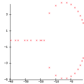
Eigenvalues plot.

Similarly, eigenvectors may be viewed with -eps_view_vectors, either in text form, in Matlab format, in binary format, or as a draw. All eigenvectors are viewed, one after the other. As an example, the next line will dump eigenvectors to the binary file evec.bin:

$ ./ex1 -n 120 -eps_nev 8 -eps_view_vectors binary:evec.bin

Two more related functions are available: EPSErrorView and EPSConvergedReasonView. These will show computed errors and the converged reason (plus number of iterations), respectively. Again, we illustrate its use via the command line. The option -eps_error_relative will show eigenvalues whose relative error are below the tolerance. The different types of errors have their corresponding options, see table Available expressions for computing error bounds.. A more detailed output can be obtained as follows:

$ ./ex1 -n 120 -eps_nev 8 -eps_error_relative ::ascii_info_detail
      ---------------------- --------------------
                 k             ||Ax-kx||/||kx||
      ---------------------- --------------------
             3.999326            1.26221e-09
             3.997304            3.82982e-10
             3.993936            2.76971e-09
             3.989224            4.94104e-10
             3.983171            6.19307e-10
             3.975781             5.9628e-10
             3.967060            2.32347e-09
             3.957012            6.12436e-09
      ---------------------- --------------------

Finally, the option for showing the converged reason is:

$ ./ex1 -n 120 -eps_nev 8 -eps_converged_reason
      Linear eigensolve converged (8 eigenpairs) due to CONVERGED_TOL; iterations 14

Advanced Usage

This section includes the description of advanced features of the eigensolver object. Default settings are appropriate for most applications and modification is unnecessary for normal usage.

Initial Guesses

In this subsection, we consider the possibility of providing initial guesses so that the eigensolver can exploit this information to get the answer faster.

Most of the algorithms implemented in EPS iteratively build and improve a basis of a certain subspace, which will eventually become an eigenspace corresponding to the wanted eigenvalues. In some solvers such as those of Krylov type, this basis is constructed starting from an initial vector, \(v_1\), whereas in other solvers such as those of Davidson type, an arbitrary subspace can be used to start the method. By default, EPS initializes the starting vector or the initial subspace randomly. This default is a reasonable choice. However, it is also possible to supply an initial subspace with the command EPSSetInitialSpace

EPSSetInitialSpace(EPS eps,PetscInt n,Vec is[]);

In some cases, a suitable initial space can accelerate convergence significantly, for instance when the eigenvalue calculation is one of a sequence of closely related problems, where the eigenspace of one problem is fed as the initial guess for the next problem.

Note that if the eigensolver supports only a single initial vector, but several guesses are provided, then all except the first one will be discarded. One could still build a vector that is rich in the directions of all guesses, by taking a linear combination of them, but this is less effective than using a solver that considers all guesses as a subspace.

Dealing with Deflation Subspaces

In some applications, when solving an eigenvalue problem the user wishes to use a priori knowledge about the solution. This is the case when an invariant subspace has already been computed (e.g., in a previous EPSSolve call) or when a basis of the null-space is known.

Consider the following example. Given a graph \(G\), with vertex set \(V\) and edges \(E\), the Laplacian matrix of \(G\) is a sparse symmetric positive semidefinite matrix \(L\) with elements

(11)\[\begin{split}l_{ij}=\left\{\begin{array}{cl} d(v_i) & \mathrm{if}\;i=j\\ -1 & \mathrm{if}\;e_{ij}\in E\\ 0&\mathrm{otherwise} \end{array}\right.\end{split}\]

where \(d(v_i)\) is the degree of vertex \(v_i\). This matrix is singular since all row sums are equal to zero. The constant vector is an eigenvector with zero eigenvalue, and if the graph is connected then all other eigenvalues are positive. The so-called Fiedler vector is the eigenvector associated with the smallest nonzero eigenvalue and can be used in heuristics for a number of graph manipulations such as partitioning. One possible way of computing this vector with SLEPc is to instruct the eigensolver to search for the smallest eigenvalue (with EPSSetWhichEigenpairs or by using a spectral transformation as described in next chapter) but preventing it from computing the already known eigenvalue. For this, the user must provide a basis for the invariant subspace (in this case just vector \([1,1,\ldots,1]^T\)) so that the eigensolver can deflate this subspace. This process is very similar to what eigensolvers normally do with invariant subspaces associated with eigenvalues as they converge. In other words, when a deflation space has been specified, the eigensolver works with the restriction of the problem to the orthogonal complement of this subspace.

The following function can be used to provide the EPS object with some basis vectors corresponding to a subspace that should be deflated during the solution process. EPSSetDeflationSpace

EPSSetDeflationSpace(EPS eps,PetscInt n,Vec defl[])

The value n indicates how many vectors are passed in argument defl.

The deflation space can be any subspace but typically it is most useful in the case of an invariant subspace or a null-space. In any case, SLEPc internally checks to see if all (or part of) the provided subspace is a null-space of the associated linear system (see section Solution of Linear Systems). In this case, this null-space is attached to the coefficient matrix of the linear solver (see PETSc’s function MatSetNullSpace) to enable the solution of singular systems. In practice, this allows the computation of eigenvalues of singular pencils (i.e., when \(A\) and \(B\) share a common null-space).

Orthogonalization

Internally, eigensolvers in EPS often need to orthogonalize a vector against a set of vectors (for instance, when building an orthonormal basis of a Krylov subspace). This operation is carried out typically by a Gram-Schmidt orthogonalization procedure. The user is able to adjust several options related to this algorithm, although the default behavior is good for most cases, and we strongly suggest not to change any of these settings. This topic is covered in detail in Hernandez et al. [2007].

Specifying a Region for Filtering

Some solvers in EPS (and other solver classes as well) can take into consideration a user-defined region of the complex plane, e.g., an ellipse. A region can be used for two purposes:

• To instruct the eigensolver to compute all eigenvalues lying in that region. This is available only in eigensolvers based on the contour integral technique (EPSCISS).

• To filter out eigenvalues outside the region. In this way, eigenvalues lying inside the region get higher priority during the iteration and are more likely to be returned as computed solutions.

Regions are specified by means of an RG object. This object is handled internally in the EPS solver, as other auxiliary objects, and can be extracted with EPSGetRG

EPSGetRG(EPS eps,RG *rg);

to set the options that define the region. These options can also be set in the command line. The following example computes largest magnitude eigenvalues, but restricting to an ellipse of radius 0.5 centered at the origin (with vertical scale 0.1):

$ ./ex1 -rg_type ellipse -rg_ellipse_center 0 -rg_ellipse_radius 0.5
                -rg_ellipse_vscale 0.1

If one wants to use the region to specify where eigenvalues should not be computed, then the region must be the complement of the specified one. The next command line computes the smallest eigenvalues not contained in the ellipse:

$ ./ex1 -eps_smallest_magnitude -rg_type ellipse -rg_ellipse_center 0
                -rg_ellipse_radius 0.5 -rg_ellipse_vscale 0.1 -rg_complement

Additional details of the RG class can be found in section Auxiliary Classes.

Computing a Large Portion of the Spectrum

We now consider the case when the user requests a relatively large number of eigenpairs (the related case of computing all eigenvalues in a given interval is addressed in section Spectrum Slicing). To fix ideas, suppose that the problem size (the dimension of the matrix, denoted as n), is in the order of 100,000’s, and the user wants nev to be approximately 5,000 (recall the notation of EPSSetDimensions in section Defining the Problem).

The first comment is that for such large values of nev, the rule of thumb suggested in section Defining the Problem for selecting the value of ncv (\(\mathtt{ncv}\geq2\cdot\mathtt{nev}\)) may be inappropriate. For small values of nev, this rule of thumb is intended to provide the solver with a sufficiently large subspace. But for large values of nev, it may be enough setting ncv to be slightly larger than nev.

The second thing to take into account has to do with costs, both in terms of storage and in terms of computational effort. This issue is dependent on the particular eigensolver used, but generally speaking the user can simplify to the following points:

1. It is necessary to store a basis of the subspace, that is, ncv vectors of length n.

2. A considerable part of the computation is devoted to orthogonalization of the basis vectors, whose cost is roughly of order \(\mathtt{ncv}^2\cdot\mathtt{n}\).

3. Within the eigensolution process, a projected eigenproblem of order ncv is built. At least one dense matrix of this dimension has to be stored.

4. Solving the projected eigenproblem has a computational cost of order \(\mathtt{ncv}^3\). Typically, such problems need to be solved many times within the eigensolver iteration.

It is clear that a large value of ncv implies a high storage requirement (points 1 and 3, especially point 1), and a high computational cost (points 2 and 4, especially point 2). However, in a scenario of such big eigenproblems, it is customary to solve the problem in parallel with many processors. In that case, it turns out that the basis vectors are stored in a distributed way and the associated operations are parallelized, so that points 1 and 2 become benign as long as sufficient processors are used. Then points 3 and 4 become really critical since in the current SLEPc version the projected eigenproblem (and its associated operations) are not treated in parallel. In conclusion, the user must be aware that using a large ncv value introduces a serial step in the computation with high cost, that cannot be amortized by increasing the number of processors.

From SLEPc 3.0.0, another parameter mpd has been introduced to alleviate this problem. The name mpd stands for maximum projected dimension. The idea is to bound the size of the projected eigenproblem so that steps 3 and 4 work with a dimension of mpd at most, while steps 1 and 2 still work with a bigger dimension, up to ncv. Suppose we want to compute nev=5000. Setting ncv=10000 or even ncv=6000 would be prohibitively expensive, for the reasons explained above. But if we set e.g. mpd=600 then the overhead of steps 3 and 4 will be considerably diminished. Of course, this reduces the potential of approximation at each outer iteration of the algorithm, but with more iterations the same result should be obtained. The benefits will be specially noticeable in the setting of parallel computation with many processors.

Note that it is not necessary to set both ncv and mpd. For instance, one can do

$ ./program -eps_nev 5000 -eps_mpd 600

Computing Interior Eigenvalues with Harmonic Extraction

The standard Rayleigh-Ritz projection procedure described in section Eigenvalue Problems is most appropriate for approximating eigenvalues located at the periphery of the spectrum, especially those of largest magnitude. Most eigensolvers in SLEPc are restarted, meaning that the projection is carried out repeatedly with increasingly good subspaces. An effective restarting mechanism, such as that implemented in Krylov-Schur, improves the subspace by realizing a filtering effect that tries to eliminate components in the direction of unwanted eigenvectors. In that way, it is possible to compute eigenvalues located anywhere in the spectrum, even in its interior.

Even though in theory eigensolvers could be able to approximate interior eigenvalues with a standard extraction technique, in practice convergence difficulties may arise that prevent success. The problem comes from the property that Ritz values (the approximate eigenvalues provided by the standard projection procedure) converge from the interior to the periphery of the spectrum. That is, the Ritz values that stabilize first are those in the periphery, so convergence of interior ones requires the previous convergence of all eigenvalues between them and the periphery. Furthermore, this convergence behaviour usually implies that restarting is carried out with bad approximations, so the restart is ineffective and global convergence is severely damaged.

Harmonic projection is a variation that uses a target value, \(\tau\), around which the user wants to compute eigenvalues (see, e.g., [Morgan and Zeng, 2006]). The theory establishes that harmonic Ritz values converge in such a way that eigenvalues closest to the target stabilize first, and also that no unconverged value is ever close to the target, so restarting is safe in this case. As a conclusion, eigensolvers with harmonic extraction may be effective in computing interior eigenvalues. Whether it works or not in practical cases depends on the particular distribution of the spectrum.

In order to use harmonic extraction in SLEPc, it is necessary to indicate it explicitly, and provide the target value as described in section Defining the Problem (default is \(\tau=0\)). The type of extraction can be set with: EPSSetExtraction

EPSSetExtraction(EPS eps,EPSExtraction extr);

Available possibilities are EPS_RITZ for standard projection and EPS_HARMONIC for harmonic projection (other alternatives such as refined extraction are still experimental).

A command line example would be:

$ ./ex5 -m 45 -eps_harmonic -eps_target 0.8 -eps_ncv 60

The example computes the eigenvalue closest to \(\tau=0.8\) of a real non-symmetric matrix of order 1035. Note that ncv has been set to a larger value than would be necessary for computing the largest magnitude eigenvalues. In general, users should expect a much slower convergence when computing interior eigenvalues compared to extreme eigenvalues. Increasing the value of ncv may help.

Currently, harmonic extraction is available in the default EPS solver, that is, Krylov-Schur, and also in Arnoldi, GD, and JD.

Balancing for Non-Hermitian Problems

In problems where the matrix has a large norm, \(\|A\|_2\), the roundoff errors introduced by the eigensolver may be large. The goal of balancing is to apply a simple similarity transformation, \(DAD^{-1}\), that keeps the eigenvalues unaltered but reduces the matrix norm, thus enhancing the accuracy of the computed eigenpairs. Obviously, this makes sense only in the non-Hermitian case. The matrix \(D\) is chosen to be diagonal, so balancing amounts to scaling the matrix rows and columns appropriately.

In SLEPc, the matrix \(DAD^{-1}\) is not formed explicitly. Instead, the operators of table Operators used in each spectral transformation mode. are preceded by a multiplication by \(D^{-1}\) and followed by a multiplication by \(D\). This allows for balancing in the case of problems with an implicit matrix.

A simple and effective Krylov balancing technique, described in [Chen and Demmel, 2000], is implemented in SLEPc. The user calls the following subroutine to activate it. EPSSetBalance

EPSSetBalance(EPS eps,EPSBalance bal,PetscInt its,PetscReal cutoff);

Two variants are available, one-sided and two-sided, and there is also the possibility for the user to provide a pre-computed \(D\) matrix.

Structured Eigenvalue Problems

Structured eigenvalue problems are those whose defining matrices are structured, i.e., their \(n^2\) entries depend on less than \(n^2\) parameters. Symmetry is the most obvious structure, and it is supported in SLEPc solvers via the EPS_HEP and EPS_GHEP problem types, see table Problem types considered in EPS.. The last entries listed in table Problem types considered in EPS. address other types of structured eigenproblems, which are discussed in this subsection. Preserving the algebraic structure can help preserve physically relevant symmetries in the eigenvalues of the matrix and may improve the accuracy and efficiency of the eigensolver. For example, in quadratic eigenvalue problems arising from gyroscopic systems (see section Quadratic Eigenvalue Problems), eigenvalues appear in quadruples \(\{\lambda,-\lambda,\bar\lambda,-\bar\lambda\}\), i.e., the spectrum is symmetric with respect to both the real and imaginary axes. This problem can be linearized to a \(2n\times 2n\) skew-Hamiltonian/Hamiltonian pencil with the same eigenvalues. A structure-preserving eigensolver will give a more accurate answer because it enforces the structure throughout the computation.

Unless otherwise stated, the structured eigenproblems discussed below are only supported in the default EPS solver, Krylov-Schur. The idea is that the user creates the structured matrix with a helper function such as MatCreateBSE (see below), and then selects the appropriate problem type with EPSSetProblemType, in this case EPS_BSE. This will instruct the solver to exploit the problem structure. Alternatively, one can solve the problem as EPS_NHEP, in which case the solver will neglect the structure.

Bethe-Salpeter

One structured eigenproblem that has raised interest recently is related to the Bethe–Salpeter equation, which is relevant in many state-of-the-art computational physics codes. For instance, in the Yambo software [Sangalli et al., 2019] it is used to evaluate optical properties. It is commonly formulated as an eigenvalue problem with a block-structured matrix,

(12)\[\begin{split}H = \begin{bmatrix} R & C \\ -C^H & -R^T \end{bmatrix},\end{split}\]

where \(R\) is Hermitian and \(C\) is complex symmetric. For a good enough approximation of the optical absorption spectrum, it is sufficient to compute a few eigenvalues with a customized version of Krylov-Schur. In this problem, eigenvalues are real and come in pairs \(\{\lambda,-\lambda\}\). The eigenvalues of interest are those with the smallest magnitude, which in this case lie in the middle of the spectrum. Usually, both right and left eigenvectors are required, but the left eigenvectors can be obtained inexpensively once the corresponding right ones are known.

The helper function to generate the matrix \(H\) of equation (12) from the blocks \(R\) and \(C\) is MatCreateBSE, and the associated problem type is EPS_BSE (or -eps_bse from the command line). It is possible to select a few variants of the solver with the function EPSKrylovSchurSetBSEType.

Further details about the implementation of the SLEPc solvers for the BSE can be found in [Alvarruiz et al., 2025].

Hamiltonian

The Hamiltonian structure is relevant in many applications, particularly in control theory. A (complex) Hamiltonian matrix has the block structure

(13)\[\begin{split}H = \begin{bmatrix} A & B \\ C & -A^* \end{bmatrix},\end{split}\]

where \(A\), \(B\) and \(C\) are either real with \(B=B^T\), \(C=C^T\), or complex with \(B=B^*\), \(C=C^*\). In the real case, eigenvalues appear in pairs \(\{\lambda,-\lambda\}\) and for complex eigenvalues in quadruples \(\{\lambda,-\lambda,\bar\lambda,-\bar\lambda\}\). For a complex Hamiltonian matrix, if \(\lambda\) is an eigenvalue, then \(-\bar\lambda\) is also an eigenvalue. A structure-preserving eigensolver has been implemented in EPS (in Krylov-Schur), which is activated by selecting the EPS_HAMILT problem type (or -eps_hamiltonian from the command line). Note that matrix \(H\) (13) must be created with the helper function MatCreateHamiltonian in order to use this solver.

Warning

The structure-preserving eigensolver for Hamiltonian eigenvalue problems should be considered experimental. Depending on the problem, it may become numerically unstable after some iterations, in which case the solver will abort, returning less eigenvalues than requested.

Footnotes

[Alvarruiz:2025:VTR]

Fernando Alvarruiz, Blanca Mellado-Pinto, and Jose E. Roman. Variants of thick-restart lanczos for the bethe-salpeter eigenvalue problem. arXiv:2503.20920 : retrieved 27 May 2025, 2025.

[Bai:2000:TSA]

Z. Bai, J. Demmel, J. Dongarra, A. Ruhe, and H. van der Vorst, editors. Templates for the Solution of Algebraic Eigenvalue Problems: A Practical Guide. Society for Industrial and Applied Mathematics, Philadelphia, PA, 2000.

[Chen:2000:BSM]

Tzu-Yi Chen and James W. Demmel. Balancing sparse matrices for computing eigenvalues. Linear Algebra and its Applications, 309(1–3):261–287, 2000.

[Golub:2000:EC2]

Gene H. Golub and Henk A. van der Vorst. Eigenvalue computation in the 20th century. Journal of Computational and Applied Mathematics, 123(1-2):35–65, 2000.

[str-1]

V. Hernandez, J. E. Roman, A. Tomas, and V. Vidal. Orthogonalization Routines in SLEPc. Technical Report STR-1, Universitat Politècnica de València, 2007. Available at https://slepc.upv.es.

[str-11]

Y. Maeda, T. Sakurai, and J. E. Roman. Contour Integral Spectrum Slicing Method in SLEPc. Technical Report STR-11, Universitat Politècnica de València, 2016. Available at https://slepc.upv.es.

[Morgan:2006:HRA]

Ronald B. Morgan and Min Zeng. A harmonic restarted Arnoldi algorithm for calculating eigenvalues and determining multiplicity. Linear Algebra and its Applications, 415(1):96–113, 2006.

[Parlett:1980:SEP]

B. N. Parlett. The Symmetric Eigenvalue Problem. Prentice-Hall, Englewood Cliffs, NJ, 1980. Reissued with revisions by SIAM, Philadelphia, 1998.

[Saad:1992:NML] (1,2)

Y. Saad. Numerical Methods for Large Eigenvalue Problems: Theory and Algorithms. John Wiley and Sons, New York, 1992.

[Sangalli:2019:MPT]

D. Sangalli, A. Ferretti, H. Miranda, C. Attaccalite, I. Marri, E. Cannuccia, P. Melo, M. Marsili, F. Paleari, A. Marrazzo, G. Prandini, P. Bonfà, M. O. Atambo, F. Affinito, M. Palummo, A. Molina-Sánchez, C. Hogan, M. Grüning, D. Varsano, and A. Marini. Many-body perturbation theory calculations using the yambo code. J. Condens. Matter Phys., 31(32):325902, 2019. doi:10.1088/1361-648x/ab15d0.

[Stewart:2001:MAV]

G. W. Stewart. Matrix Algorithms. Volume II: Eigensystems. Society for Industrial and Applied Mathematics, Philadelphia, PA, USA, 2001.

---

[1] (1,2)

If SLEPc is compiled for real scalars, then the absolute value of the imaginary part, \(\|\mathrm{Im}(\lambda)\|\), is used for eigenvalue selection and sorting.

References

F. Alvarruiz, B. Mellado-Pinto, and J. E. Roman. Variants of thick-restart Lanczos for the Bethe-Salpeter eigenvalue problem. arXiv:2503.20920 : retrieved 27 May 2025, 2025. doi:10.48550/arXiv.2503.20920.